# A tibble: 24 × 4
   Admit    Gender Dept      n
   <chr>    <chr>  <chr> <dbl>
 1 Admitted Male   A       512
 2 Rejected Male   A       313
 3 Admitted Female A        89
 4 Rejected Female A        19
 5 Admitted Male   B       353
 6 Rejected Male   B       207
 7 Admitted Female B        17
 8 Rejected Female B         8
 9 Admitted Male   C       120
10 Rejected Male   C       205
# ℹ 14 more rows
It contains data on applicants to graduate school at Berkeley for the six largest departments in 1973 classified by admission and sex. Let’s see whether there is an association between Gender and Admit. Let’s first aggregate over department:
# A tibble: 2 × 2
  Gender `Admission rate`
  <chr>             <dbl>
1 Female            0.304
2 Male              0.445
This suggests that men have substantially higher admission rates than women. Let’s see if we can confirm this using either a Fisher’s exact test or a Pearson chi-square test.
# first convert to 2x2 table formatadmit_vs_gender <- ucb_data_agg |>pivot_wider(names_from = Gender, values_from = n) |>column_to_rownames(var ="Admit")admit_vs_gender
         Female Male
Admitted    557 1198
Rejected   1278 1493
# Fisher exact test (note that the direction of the effect can be deduced)fisher.test(admit_vs_gender)
    Fisher's Exact Test for Count Data

data:  admit_vs_gender
p-value < 2.2e-16
alternative hypothesis: true odds ratio is not equal to 1
95 percent confidence interval:
 0.4781839 0.6167675
sample estimates:
odds ratio
 0.5432254
# Chi-square testchisq.test(admit_vs_gender)
    Pearson's Chi-squared test with Yates' continuity correction

data:  admit_vs_gender
X-squared = 91.61, df = 1, p-value < 2.2e-16
As a sanity check, let’s run the Poisson regression underlying the chi-square test above.
Indeed, it does seem that female applicants typically applied to more selective departments! This suggests that it is very important to control for department when evaluating the association between admissions and gender. To do this, we can run a test for conditional independence in the \(J \times K \times L\) table:
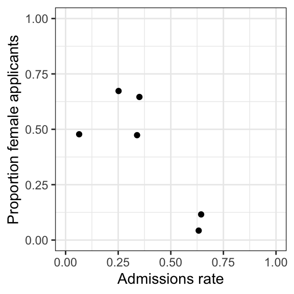
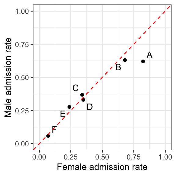
Still we find a significant effect! But what is the direction of the effect? The chi-square test does not tell us. We can simply compute the admissions rates by department and plot them:
Now the difference doesn’t seem so huge, with most departments close to even and with department A heavily skewed towards admitting women!
27.2 Revisiting the crime data, again
library(tidyverse)
Here we are again, face to face with the crime data, with one last chance to get the analysis right. Let’s load and preprocess it, as before.
# read crime datacrime_data <-read_tsv("data/Statewide_crime.dat")# read and transform population datapopulation_data <-read_csv("data/state-populations.csv")population_data <- population_data |>filter(State !="Puerto Rico") |>select(State, Pop) |>rename(state_name = State, state_pop = Pop)# collate state abbreviationsstate_abbreviations <-tibble(state_name = state.name,state_abbrev = state.abb) |>add_row(state_name ="District of Columbia", state_abbrev ="DC")# add CrimeRate to crime_datacrime_data <- crime_data |>mutate(STATE =ifelse(STATE =="IO", "IA", STATE)) |>rename(state_abbrev = STATE) |>filter(state_abbrev !="DC") |># remove outlierleft_join(state_abbreviations, by ="state_abbrev") |>left_join(population_data, by ="state_name") |>select(state_abbrev, Violent, Metro, HighSchool, Poverty, state_pop)crime_data
# A tibble: 50 × 6
   state_abbrev Violent Metro HighSchool Poverty state_pop
   <chr>          <dbl> <dbl>      <dbl>   <dbl>     <dbl>
 1 AK               593  65.6       90.2     8      724357
 2 AL               430  55.4       82.4    13.7   4934193
 3 AR               456  52.5       79.2    12.1   3033946
 4 AZ               513  88.2       84.4    11.9   7520103
 5 CA               579  94.4       81.3    10.5  39613493
 6 CO               345  84.5       88.3     7.3   5893634
 7 CT               308  87.7       88.8     6.4   3552821
 8 DE               658  80.1       86.5     5.8    990334
 9 FL               730  89.3       85.9     9.7  21944577
10 GA               454  71.6       85.2    10.8  10830007
# ℹ 40 more rows
Let’s recall the logistic regression we ran on these data in Chapter 4:
bin_fit <-glm(Violent / state_pop ~ Metro + HighSchool + Poverty,weights = state_pop,family ="binomial",data = crime_data)
We had found very poor results from the goodness of fit test for this model. We have therefore omitted some important variables and/or we have serious overdispersion on our hands.
We haven’t discussed in any detail how to deal with overdispersion in logistic regression models, so let’s try a Poisson model instead. The natural way to model rates using Poisson distributions is via offsets:
pois_fit <-glm(Violent ~ Metro + HighSchool + Poverty +offset(log(state_pop)),family ="poisson",data = crime_data)summary(pois_fit)
Call:
glm(formula = Violent ~ Metro + HighSchool + Poverty + offset(log(state_pop)),
    family = "poisson", data = crime_data)

Coefficients:
              Estimate Std. Error z value Pr(>|z|)
(Intercept) -1.609e+01  3.520e-01  -45.72   <2e-16 ***
Metro       -2.585e-02  5.727e-04  -45.15   <2e-16 ***
HighSchool   9.106e-02  3.450e-03   26.39   <2e-16 ***
Poverty      6.077e-02  4.852e-03   12.53   <2e-16 ***
---
Signif. codes:  0 '***' 0.001 '**' 0.01 '*' 0.05 '.' 0.1 ' ' 1

(Dispersion parameter for poisson family taken to be 1)

    Null deviance: 15589  on 49  degrees of freedom
Residual deviance: 11741  on 46  degrees of freedom
AIC: 12135

Number of Fisher Scoring iterations: 5
Again, everything is significant, and again, the regression summary shows that we have a huge residual deviance. This was to be expected, given that \(\text{Bin}(m, \pi) \approx \text{Poi}(m\pi)\) for large \(m\) and small \(\pi\). So, the natural thing to try is a negative binomial regression! Negative binomial regression is not implemented in the regular glm package, but glm.nb() from the MASS package is a dedicated function for this task. Let’s see what we get:
nb_fit <- MASS::glm.nb(Violent ~ Metro + HighSchool + Poverty +offset(log(state_pop)),data = crime_data)summary(nb_fit)
Call:
MASS::glm.nb(formula = Violent ~ Metro + HighSchool + Poverty +
    offset(log(state_pop)), data = crime_data, init.theta = 1.467747388,
    link = log)

Coefficients:
              Estimate Std. Error z value Pr(>|z|)
(Intercept) -10.254088   5.273418  -1.944   0.0518 .
Metro        -0.012188   0.008518  -1.431   0.1525
HighSchool    0.028052   0.052482   0.535   0.5930
Poverty      -0.026852   0.068449  -0.392   0.6948
---
Signif. codes:  0 '***' 0.001 '**' 0.01 '*' 0.05 '.' 0.1 ' ' 1

(Dispersion parameter for Negative Binomial(1.4677) family taken to be 1)

    Null deviance: 59.516  on 49  degrees of freedom
Residual deviance: 55.487  on 46  degrees of freedom
AIC: 732.58

Number of Fisher Scoring iterations: 1

              Theta:  1.468
          Std. Err.:  0.268

 2 x log-likelihood:  -722.575
Aha! Things are not looking so significant anymore! And the residual deviance is not as huge! Although, we must be careful! The residual deviance no longer has the usual \(\chi^2\) distribution because of the estimated dispersion parameter. So we don’t really have an easy goodness of fit test. The estimated value of \(\gamma\) (confusingly called \(\theta\) in the summary) is significantly different from zero, indicating overdispersion. Let’s formally test for overdispersion using the nonstandard likelihood ratio test discussed above:
So at the very least the NB model fits much better than the Poisson model. Let’s do some inference based on this model. For example, we can get Wald confidence intervals:
confint.default(nb_fit)
                   2.5 %      97.5 %
(Intercept) -20.58979658 0.081620714
Metro        -0.02888413 0.004507747
HighSchool   -0.07481066 0.130915138
Poverty      -0.16100973 0.107305015
Or we can get LRT-based (i.e. profile) confidence intervals:
confint(nb_fit)
Waiting for profiling to be done...
                   2.5 %       97.5 %
(Intercept) -19.20209590 -0.860399348
Metro        -0.03153902  0.006365841
HighSchool   -0.06265118  0.115318303
Poverty      -0.13930110  0.085200541
Or we can get confidence intervals for the predicted means:
$fit
       AK        AL        AR        AZ        CA        CO        CT        DE
 116.1520  617.7064  375.4895  700.6931 3257.5300  725.1538  436.7863  127.2572
       FL        GA        HI        ID        IL        IN        IA        KS
2232.2308 1301.2937  157.1416  263.8572 1379.1847  954.3366  546.5503  439.0649
       KY        LA        MA        MD        ME        MI        MN        MO
 541.5706  391.6745  747.7454  737.0032  274.2879 1322.9956  970.4078  871.2829
       MS        MT        NC        ND        NE        NH        NJ        NM
 380.6756  199.4947 1313.0904  134.8128  305.0634  261.1975  966.9940  204.3311
       NV        NY        OH        OK        OR        PA        RI        SC
 327.7316 1926.3861 1477.1713  495.9711  517.8397 1600.0813   96.3565  684.9102
       SD        TN        TX        UT        VA        VT        WA        WI
 160.9225  867.0224 2423.0647  416.6648 1244.5168  148.1635 1012.1932  892.0644
       WV        WY
 226.4515  100.1906

$se.fit
       AK        AL        AR        AZ        CA        CO        CT        DE
 21.00552 143.65071 130.44272 165.08459 910.57769 121.34777  85.53768  32.15169
       FL        GA        HI        ID        IL        IN        IA        KS
427.89514 173.04544  31.73873  40.28262 239.43324 147.21049 104.05752  68.82044
       KY        LA        MA        MD        ME        MI        MN        MO
133.28938 129.40665 150.23524 158.93816  92.04222 171.28409 216.32477 110.88843
       MS        MT        NC        ND        NE        NH        NJ        NM
138.28105  65.60335 379.90855  26.74061  69.62560  66.73731 220.88371  59.26953
       NV        NY        OH        OK        OR        PA        RI        SC
 64.30971 387.25204 241.24541  95.44911  81.97419 220.42078  33.97964 119.45174
       SD        TN        TX        UT        VA        VT        WA        WI
 41.50215 169.68896 738.95321 107.62725 209.14651  51.32810 191.75629 137.35158
       WV        WY
 71.55328  22.79279

$residual.scale
[1] 1
We can carry out some hypothesis tests as well, e.g. to test \(H_0: \beta_{\text{Metro}} = 0\):
Likelihood ratio tests of Negative Binomial Models

Response: Violent
                                                  Model    theta Resid. df
1         HighSchool + Poverty + offset(log(state_pop)) 1.428675        47
2 Metro + HighSchool + Poverty + offset(log(state_pop)) 1.467747        46
     2 x log-lik.   Test    df LR stat.   Pr(Chi)
1       -724.1882
2       -722.5753 1 vs 2     1 1.612878 0.2040877