# A tibble: 50 × 6
   state_abbrev CrimeRate Metro HighSchool Poverty state_pop
   <chr>            <dbl> <dbl>      <dbl>   <dbl>     <dbl>
 1 AK           0.000819   65.6       90.2     8      724357
 2 AL           0.0000871  55.4       82.4    13.7   4934193
 3 AR           0.000150   52.5       79.2    12.1   3033946
 4 AZ           0.0000682  88.2       84.4    11.9   7520103
 5 CA           0.0000146  94.4       81.3    10.5  39613493
 6 CO           0.0000585  84.5       88.3     7.3   5893634
 7 CT           0.0000867  87.7       88.8     6.4   3552821
 8 DE           0.000664   80.1       86.5     5.8    990334
 9 FL           0.0000333  89.3       85.9     9.7  21944577
10 GA           0.0000419  71.6       85.2    10.8  10830007
# ℹ 40 more rows
We can fit a GLM using the glm command, specifying as additional arguments the observation weights as well as the exponential dispersion model. In this case, the weights are the state populations and the family is binomial:
glm_fit <-glm(CrimeRate ~ Metro + HighSchool + Poverty,weights = state_pop,family ="binomial",data = crime_data)
We can print the summary table as usual:
summary(glm_fit)
Call:
glm(formula = CrimeRate ~ Metro + HighSchool + Poverty, family = "binomial",
    data = crime_data, weights = state_pop)

Coefficients:
              Estimate Std. Error z value Pr(>|z|)
(Intercept) -1.609e+01  3.520e-01  -45.72   <2e-16 ***
Metro       -2.586e-02  5.727e-04  -45.15   <2e-16 ***
HighSchool   9.106e-02  3.450e-03   26.39   <2e-16 ***
Poverty      6.077e-02  4.852e-03   12.53   <2e-16 ***
---
Signif. codes:  0 '***' 0.001 '**' 0.01 '*' 0.05 '.' 0.1 ' ' 1

(Dispersion parameter for binomial family taken to be 1)

    Null deviance: 15590  on 49  degrees of freedom
Residual deviance: 11742  on 46  degrees of freedom
AIC: 12136

Number of Fisher Scoring iterations: 5
Amazingly, everything is very significant! This is because the weights for each observation (the state populations) are very high, effectively making the sample size very high. But frankly, this is a bit suspicious. Glancing at the bottom of the regression summary, we see a residual deviance of 11742 on 46 degrees of freedom. This part of the summary refers to the deviance-based goodness of fit test. Under the null hypothesis that the model fits well, we expect that the residual deviance has a distribution of \(\chi^2_{46}\), which has a mean of 46.
Let’s formally check the goodness of fit. We can extract the residual deviance and residual degrees of freedom from the GLM fit:
glm_fit$deviance
[1] 11742.28
glm_fit$df.residual
[1] 46
We can then compute the chi-square \(p\)-value:
# compute based on residual deviance from fit objectpchisq(glm_fit$deviance,df = glm_fit$df.residual,lower.tail =FALSE)
[1] 0
# compute residual deviance as sum of squares of residualspchisq(sum(resid(glm_fit, "deviance")^2),df = glm_fit$df.residual,lower.tail =FALSE)
[1] 0
Wow, we get a \(p\)-value of zero! Let’s try doing a score-based (i.e., Pearson) goodness of fit test:
Also zero. So we need to immediately stop using this model for inference about these data, since it fits the data very poorly. We will discuss how to build a better model for the crime data in the next unit. For now, we turn to analyzing a different dataset.
23.2 Noisy miner data
Credit: Generalized Linear Models With Examples in R textbook.
Let’s consider the noisy miner dataset. Noisy miners are a small but aggressive native Australian bird. We want to know how the number of these birds observed in a patch of land depends on various factors of that patch of land.
Still, there is some model misspecification, but for now, we still proceed with the rest of the analysis.
The standard errors shown in the summary are based on the Wald test. We can get Wald confidence intervals based on these standard errors by using the formula:
We see that the prediction on the linear predictor scale is exactly the logarithm of the prediction on the mean scale. However, the standard error given on the mean scale uses the delta method. We prefer to directly transform the confidence interval from the linear scale using the inverse link function (in this case, the exponential):
# using delta methodc(pred_mean$fit +qnorm(0.025)*pred_mean$se.fit, pred_mean$fit +qnorm(0.975)*pred_mean$se.fit)
       31        31
0.9312839 2.9216197
# using transformationexp(c(pred_linear$fit +qnorm(0.025)*pred_linear$se.fit, pred_linear$fit +qnorm(0.975)*pred_linear$se.fit))
      31       31
1.149238 3.229285
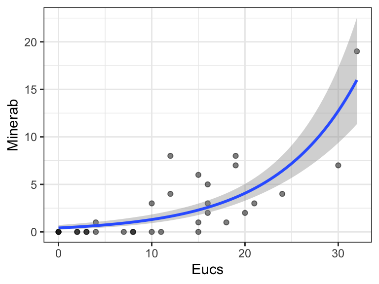
In this case, the intervals obtained are somewhat different. We can plot confidence intervals for the fit in a univariate case (e.g., regressing Minerab on Eucs) using geom_smooth():
We can also test the coefficients in the model. The Wald tests for individual coefficients were already given by the regression summary above. We might want to carry out likelihood ratio tests for individual coefficients instead. For example, let’s do this for Eucs:
glm_fit_partial <-glm(Minerab ~ . - Miners - Eucs, family ="poisson", data = nminer)anova(glm_fit_partial, glm_fit, test ="LRT")