2 Interpreting linear models
2.1 Predictors and coefficients
See also Agresti 1.2, Dunn and Smyth 1.4, 1.7, 2.7
The types of predictors \(x_j\) (e.g. binary or continuous) has less of an effect on the regression than the type of response, but it is still important to pay attention to the former.
Intercepts. It is common to include an intercept in a linear regression model, a predictor \(x_0\) such that \(x_{i0} = 1\) for all \(i\). When an intercept is present, we index it as the 0th predictor. The simplest kind of linear model is the intercept-only model or the one-sample model: \[ y = \beta_0 + \epsilon. \tag{2.1}\] The parameter \(\beta_0\) is the mean of the response.
Binary predictors. In addition to an intercept, suppose we have a binary predictor \(x_1 \in \{0,1\}\) (e.g. \(x_1 = 1\) for patients who took blood pressure medication and \(x_1 = 0\) for those who didn’t). This leads to the following linear model: \[ y = \beta_0 + \beta_1 x_1 + \epsilon. \tag{2.2}\] Here, \(\beta_0\) is the mean response (say blood pressure) for observations with \(x_1 = 0\) and \(\beta_0 + \beta_1\) is the mean response for observations with \(x_1 = 1\). Therefore, the parameter \(\beta_1\) is the difference in mean response between observations with \(x_1 = 1\) and \(x_1 = 0\). This parameter is sometimes called the effect or effect size of \(x_1\), though a causal relationship might or might not be present. The model (2.2) is sometimes called the two-sample model, because the response data can be split into two “samples”: those corresponding to \(x_1 = 0\) and those corresponding to \(x_1 = 1\).
Categorical predictors. A binary predictor is a special case of a categorical predictor: A predictor taking two or more discrete values. Suppose we have a predictor \(w \in \{w_0, w_1, \dots, w_{C-1}\}\), where \(C \geq 2\) is the number of categories and \(w_0, \dots, w_{C-1}\) are the levels of \(w\). E.g. suppose \(\{w_0, \dots, w_{C-1}\}\) is the collection of U.S. states, so that \(C = 50\). If we want to regress a response on the categorical predictor \(w\), we cannot simply set \(x_1 = w\) in the context of the linear regression (2.2). Indeed, \(w\) does not necessarily take numerical values. Instead, we need to add a predictor \(x_j\) for each of the levels of \(w\). In particular, define \(x_j \equiv 1(w = w_j)\) for \(j = 1, \dots, C-1\) and consider the regression \[ y = \beta_0 + \beta_1 x_1 + \cdots + \beta_{C-1}x_{C-1} + \epsilon. \tag{2.3}\] Here, category 0 is the base category, and \(\beta_0\) represents the mean response in the base category. The coefficient \(\beta_j\) represents the difference in mean response between the \(j\)th category and the base category.
Quantitative predictors. A quantitative predictor is one that can take on any real value. For example, suppose that \(x_1 \in \mathbb{R}\), and consider the linear model \[ y = \beta_0 + \beta_1 x_1 + \epsilon. \tag{2.4}\] Now, the interpretation of \(\beta_1\) is that an increase in \(x_1\) by 1 is associated with an increase in \(y\) by \(\beta_1\). We must be careful to avoid saying “an increase in \(x_1\) by 1 causes \(y\) to increase by \(\beta_1\)” unless we make additional causal assumptions. Note that the units of \(x_1\) matter. If \(x_1\) is the height of a person, then the value and the interpretation of \(\beta_1\) changes depending on whether that height is measured in feet or in meters.
Ordinal predictors. There is an awkward category of predictor in between categorical and continuous called ordinal. An ordinal predictor is one that takes a discrete number of values, but these values have an intrinsic ordering, e.g. \(x_1 \in \{\texttt{small}, \texttt{medium}, \texttt{large}\}\). It can be treated as categorical at the cost of losing the ordering information, or as continuous if one is willing to assign quantitative values to each category.
Multiple predictors. A linear regression need not contain just one predictor (aside from an intercept). For example, let’s say \(x_1\) and \(x_2\) are two predictors. Then, a linear model with both predictors is \[ y = \beta_0 + \beta_1 x_1 + \beta_2 x_2 + \epsilon. \tag{2.5}\] When there are multiple predictors, the interpretation of coefficients must be revised somewhat. For example, \(\beta_1\) in the above regression is the effect of an increase in \(x_1\) by 1 while holding \(x_2\) constant or while adjusting for \(x_2\) or while controlling for \(x_2\). If \(y\) is blood pressure, \(x_1\) is a binary predictor indicating blood pressure medication taken and \(x_2\) is sex, then \(\beta_1\) is the effect of the medication on blood pressure while controlling for sex. In general, the coefficient of a predictor depends on what other predictors are in the model. As an extreme case, suppose the medication has no actual effect, but that men generally have higher blood pressure and higher rates of taking the medication. Then, the coefficient \(\beta_1\) in the single regression model (2.2) would be nonzero but the coefficient in the multiple regression model (2.5) would be equal to zero. In this case, sex acts as a confounder.
Interactions. Note that the multiple regression model (2.5) has the built-in assumption that the effect of \(x_1\) on \(y\) is the same for any fixed value of \(x_2\) (and vice versa). In some cases, the effect of one variable on the response may depend on the value of another variable. In this case, it’s appropriate to add another predictor called an interaction. Suppose \(x_2\) is quantitative (e.g. years of job experience) and \(x_2\) is binary (e.g. sex, with \(x_2 = 1\) meaning male). Then, we can define a third predictor \(x_3\) as the product of the first two, i.e. \(x_3 = x_1x_2\). This gives the regression model \[ y = \beta_0 + \beta_1 x_1 + \beta_2 x_2 + \beta_3 x_1 x_2 + \epsilon. \tag{2.6}\] Now, the effect of adding another year of job experience is \(\beta_1\) for females and \(\beta_1 + \beta_3\) for males. The coefficient \(\beta_3\) is the difference in the effect of job experience between males and females.
2.2 Linear model spaces
See also Agresti 1.3-1.4, Dunn and Smyth 2.1, 2.2, 2.5.1
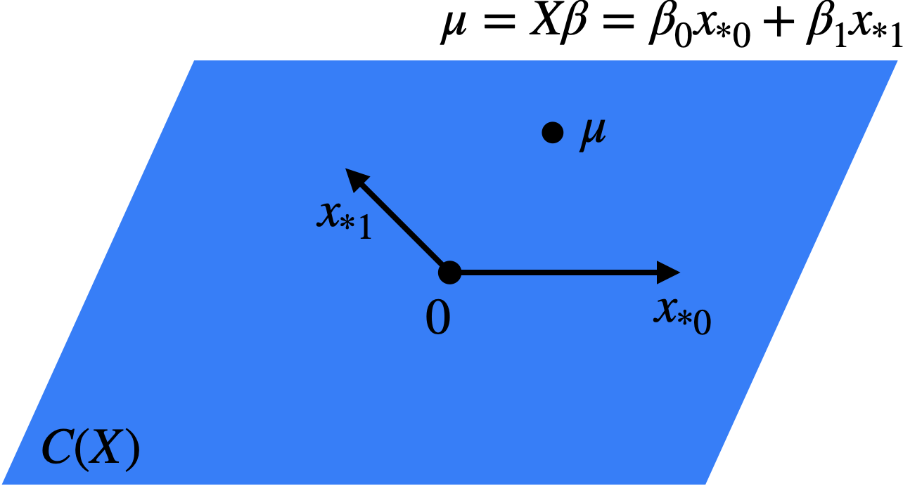
The matrix \(\boldsymbol{X}\) is called the model matrix or the design matrix. Concatenating the linear model equations across observations gives us an equivalent formulation: \[ \boldsymbol{y} = \boldsymbol{X} \boldsymbol{\beta} + \boldsymbol{\epsilon}; \quad \mathbb{E}[\boldsymbol{\epsilon}] = \boldsymbol{0}, \ \text{Var}[\boldsymbol{\epsilon}] = \sigma^2 \boldsymbol{I_n} \] or \[ \mathbb{E}[\boldsymbol{y}] = \boldsymbol{X} \boldsymbol{\beta} = \boldsymbol{\mu}. \] As \(\boldsymbol{\beta}\) varies in \(\mathbb{R}^p\), the set of possible vectors \(\boldsymbol{\mu} \in \mathbb{R}^n\) is defined \[ C(\boldsymbol{X}) \equiv \{\boldsymbol{\mu} = \boldsymbol{X} \boldsymbol{\beta}: \boldsymbol{\beta} \in \mathbb{R}^p\}. \] \(C(\boldsymbol{X})\), called the model vector space, is a subspace of \(\mathbb{R}^n\): \(C(\boldsymbol{X}) \subseteq \mathbb{R}^n\). Since \[ \boldsymbol{X} \boldsymbol{\beta} = \beta_0 \boldsymbol{x_{*0}} + \cdots + \beta_{p-1} \boldsymbol{x_{*p-1}}, \] the model vector space is the column space of the matrix \(\boldsymbol{X}\) (Figure 2.1).
The dimension of \(C(\boldsymbol{X})\) is the rank of \(\boldsymbol{X}\), i.e. the number of linearly independent columns of \(\boldsymbol{X}\). If \(\text{rank}(\boldsymbol{X}) < p\), this means that there are two different vectors \(\boldsymbol{\beta}\) and \(\boldsymbol{\beta'}\) such that \(\boldsymbol{X} \boldsymbol{\beta} = \boldsymbol{X} \boldsymbol{\beta'}\). Therefore, we have two values of the parameter vector that give the same model for \(\boldsymbol{y}\). This makes \(\boldsymbol{\beta}\) not identifiable, and makes it impossible to reliably determine \(\boldsymbol{\beta}\) based on the data. For this reason, we will generally assume that \(\boldsymbol{\beta}\) is identifiable, i.e. \(\boldsymbol{X} \boldsymbol{\beta} \neq \boldsymbol{X} \boldsymbol{\beta'}\) if \(\boldsymbol{\beta} \neq \boldsymbol{\beta'}\). This is equivalent to the assumption that \(\text{rank}(\boldsymbol{X}) = p\). Note that this cannot hold when \(p > n\), so for the majority of the course we will assume that \(p \leq n\). In this case, \(\text{rank}(\boldsymbol{X}) = p\) if and only if \(\boldsymbol{X}\) has full-rank.
As an example when \(p \leq n\) but when \(\boldsymbol{\beta}\) is still not identifiable, consider the case of a categorical predictor. Suppose the categories of \(w\) were \(\{w_1, \dots, w_{C-1}\}\), i.e. the baseline category \(w_0\) did not exist. In this case, the model (2.3) would not be identifiable because \(x_0 = 1 = x_1 + \cdots + x_{C-1}\) and thus \(x_{*0} = 1 = x_{*1} + \cdots + x_{*,C-1}\). Indeed, this means that one of the predictors can be expressed as a linear combination of the others, so \(\boldsymbol{X}\) cannot have full rank. A simpler way of phrasing the problem is that we are describing \(C-1\) intrinsic parameters (the means in each of the \(C-1\) groups) with \(C\) model parameters. There must therefore be some redundancy. For this reason, if we include an intercept term in the model then we must designate one of our categories as the baseline and exclude its indicator from the model.