4 Analysis of variance
See also Agresti 2.4.2, 2.4.3, 2.4.6, Dunn and Smyth 2.9
4.1 Analysis of variance
The orthogonality property of least squares, together with the Pythagorean theorem, leads to a fundamental relationship called the analysis of variance.
Let’s say that \(S \subset \{0, 1, \dots, p-1\}\) is a subset of the predictors we wish to exclude from the model. First regress \(\boldsymbol{y}\) on \(\boldsymbol{X}\) to get \(\boldsymbol{\widehat{\beta}}\) as usual. Then, we consider the partial model matrix \(\boldsymbol{X_{*,\text{-}S}}\) obtained by selecting all predictors except those in \(S\). Regressing \(\boldsymbol{y}\) on \(\boldsymbol{X_{*, \text{-}S}}\) results in \(\boldsymbol{\widehat{\beta}_{\text{-}S}}\) (note: \(\boldsymbol{\widehat{\beta}_{\text{-}S}}\) is not necessarily obtained from \(\boldsymbol{\widehat{\beta}}\) by extracting the coefficients corresponding to \(\text{-}S\)).
Theorem 4.1 \[ \|\boldsymbol{y} - \boldsymbol{X_{*, \text{-}S}}\boldsymbol{\widehat{\beta}_{\text{-}S}}\|^2 = \|\boldsymbol{X}\boldsymbol{\widehat{\beta}} - \boldsymbol{X_{*, \text{-}S}}\boldsymbol{\widehat{\beta}_{\text{-}S}}\|^2 + \|\boldsymbol{y} - \boldsymbol{X}\boldsymbol{\widehat{\beta}}\|^2. \tag{4.1}\]
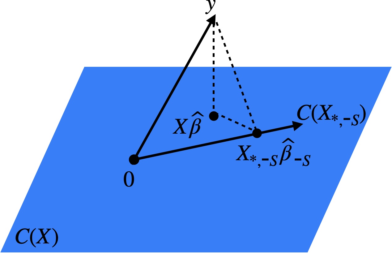
Proof. Consider the three points \(\boldsymbol{y}\), \(\boldsymbol{X}\boldsymbol{\widehat{\beta}}\), \(\boldsymbol{X_{*, \text{-}S}}\boldsymbol{\widehat{\beta}_{\text{-}S}} \in \mathbb{R}^n\). Since \(\boldsymbol{X}\boldsymbol{\widehat{\beta}}\) and \(\boldsymbol{X_{*, \text{-}S}}\boldsymbol{\widehat{\beta}_{\text{-}S}}\) are both in \(C(\boldsymbol{X})\), it follows by the orthogonal projection property that \(\boldsymbol{y} - \boldsymbol{X}\boldsymbol{\widehat{\beta}}\) is orthogonal to \(\boldsymbol{X}\boldsymbol{\widehat{\beta}} - \boldsymbol{X_{*, \text{-}S}}\boldsymbol{\widehat{\beta}_{\text{-}S}}\). In other words, these three points form a right triangle (Figure 4.1). The relationship (4.1) is then a consequence of the Pythagorean theorem.
We will rely on this fundamental relationship throughout this course. One important special case is when \(S = \{1, \dots, p-1\}\), i.e., the model without \(S\) is the intercept-only model. In this case, \(\boldsymbol{X_{*, \text{-}S}} = \boldsymbol{1_n}\) and \(\boldsymbol{\widehat{\beta}_{\text{-}S}} = \bar{y}\). Therefore, equation (4.1) implies the following.
Proposition 4.1 \[ \|\boldsymbol{y} - \bar{y} \boldsymbol{1_n}\|^2 = \|\boldsymbol{X}\boldsymbol{\widehat{\beta}} - \bar{y} \boldsymbol{1_n}\|^2 + \|\boldsymbol{y} - \boldsymbol{X}\boldsymbol{\widehat{\beta}}\|^2. \]
Equivalently, we can rewrite this equation as follows:
\[ \textnormal{SST} \equiv \sum_{i = 1}^n (y_i - \bar{y})^2 = \sum_{i = 1}^n (\widehat{\mu}_i - \bar{y})^2 + \sum_{i = 1}^n (y_i - \widehat{\mu}_i)^2 \equiv \textnormal{SSR} + \textnormal{SSE}. \tag{4.2}\]
4.2 \(R^2\) and multiple correlation
The ANOVA decomposition (4.2) of the variation in \(\boldsymbol{y}\) into that explained by the linear regression model (SSR) and that left over (SSE) leads naturally to the definition of \(R^2\) as the fraction of variation in \(\boldsymbol{y}\) explained by the linear regression model:
\[ R^2 \equiv \frac{\text{SSR}}{\text{SST}} = \frac{\sum_{i = 1}^n (\widehat{\mu}_i - \bar{y})^2}{\sum_{i = 1}^n (y_i - \bar{y})^2} = \frac{\|\boldsymbol{X}\boldsymbol{\widehat{\beta}} - \bar{y} \boldsymbol{1_n}\|^2}{\|\boldsymbol{y} - \bar{y} \boldsymbol{1_n}\|^2}. \]
By the decomposition (4.2), we have \(R^2 \in [0,1]\). The closer \(R^2\) is to 1, the more closely the data follow the fitted linear regression model. This intuition is formalized in the following result.
Proposition 4.2 \(R^2\) is the squared sample correlation between \(\boldsymbol{X} \boldsymbol{\widehat{\beta}}\) and \(\boldsymbol{y}\).
For this reason, the positive square root of \(R^2\) is called the multiple correlation coefficient.
Proof. The first step is to observe that the mean of \(\boldsymbol{X} \boldsymbol{\widehat{\beta}}\) is \(\bar{y}\) (this follows from the normal equations). Therefore, the sample correlation between \(\boldsymbol{X} \boldsymbol{\widehat{\beta}}\) and \(\boldsymbol{y}\) is the inner product of the unit-normalized vectors \(\boldsymbol{X} \boldsymbol{\widehat{\beta}} - \bar{y} \boldsymbol{1}\) and \(\boldsymbol{y} - \bar{y} \boldsymbol{1}\), which is the cosine of the angle between them. From the geometry of Figure 4.1, we find that the cosine of the angle between \(\boldsymbol{X} \boldsymbol{\widehat{\beta}} - \bar{y} \boldsymbol{1}\) and \(\boldsymbol{y} - \bar{y} \boldsymbol{1}\) is \(\|\boldsymbol{X} \boldsymbol{\widehat{\beta}} - \bar{y} \boldsymbol{1}\|/\|\boldsymbol{y} - \bar{y} \boldsymbol{1}\|\). Squaring this relation gives the desired conclusion.
4.3 \(R^2\) increases as predictors are added
The \(R^2\) is an in-sample measure, i.e., it uses the same data to fit the model and to assess the quality of the fit. Therefore, it is generally an optimistic measure of the (out-of-sample) prediction error. One manifestation of this is that the \(R^2\) increases if any predictors are added to the model (even if these predictors are “junk”). To see this, it suffices to show that SSE decreases as we add predictors. Without loss of generality, suppose that we start with a model with all predictors except those in \(S \subset \{0, 1, \dots, p-1\}\) and compare it to the model including all the predictors \(\{0,1,\dots,p-1\}\). We can read off from the Pythagorean theorem (4.1) that:
\[ \text{SSE}(\boldsymbol{X_{*, \text{-}S}}, \boldsymbol{y}) \equiv \|\boldsymbol{y} - \boldsymbol{X_{*, \text{-}S}}\boldsymbol{\widehat{\beta}_{\text{-}S}}\|^2 \geq \|\boldsymbol{y} - \boldsymbol{X}\boldsymbol{\widehat{\beta}}\|^2 \equiv \text{SSE}(\boldsymbol{X}, \boldsymbol{y}). \]
Adding many junk predictors will have the effect of degrading predictive performance but will nevertheless increase \(R^2\).
4.4 Special cases
4.4.1 The \(C\)-groups model
See also Agresti 2.3.2-2.3.3
4.4.1.1 ANOVA decomposition for \(C\) groups model
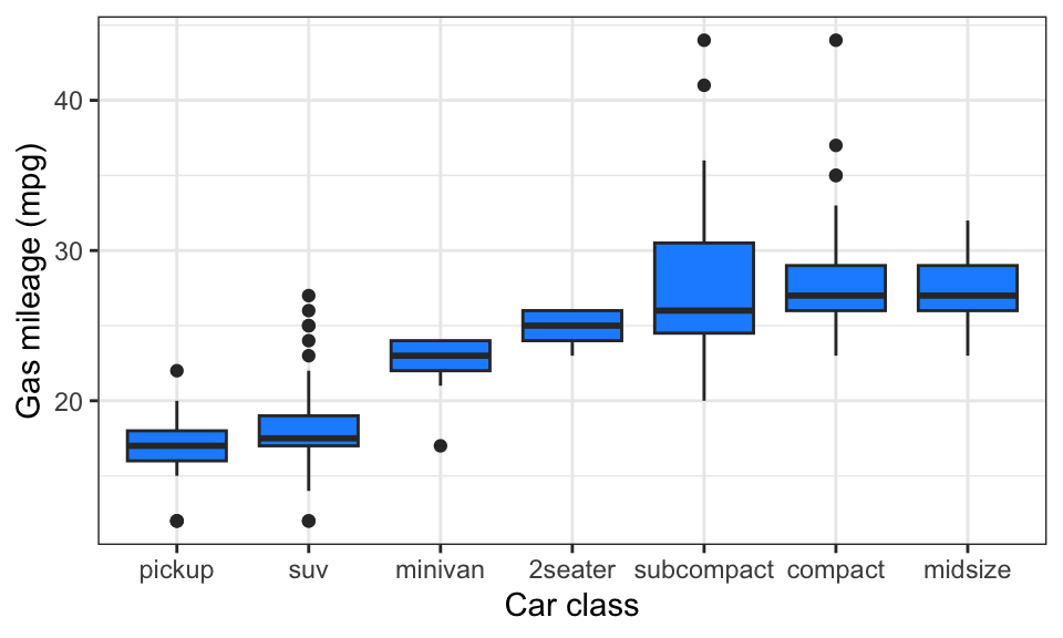
Let’s consider the special case of the ANOVA decomposition (4.2) when the model matrix \(\boldsymbol{X}\) represents a single categorical predictor \(w\). In this case, each observation \(i\) is associated with one of the \(C\) classes of \(w\), which we denote \(c(i) \in \{1, \dots, C\}\). Let’s consider the \(C\) groups of observations \(\{i: c(i) = c\}\) for \(c \in \{1, \dots, C\}\). For example, \(w\) may be the type of a car (compact, midsize, minivan, etc.) and \(y\) might be its fuel efficiency in miles per gallon.
It is easy to check that the least squares fitted values \(\widehat{\mu}_i\) are simply the means of the corresponding groups:
\[ \widehat{\mu}_i = \bar{y}_{c(i)}, \quad \text{where}\ \bar{y}_{c(i)} \equiv \frac{\sum_{i: c(i) = c} y_i}{|\{i: c(i) = c\}|}. \]
Therefore, we have:
\[ \text{SSR} = \sum_{i = 1}^n (\widehat{\mu}_i - \bar{y})^2 = \sum_{i = 1}^n (\bar{y}_{c(i)} - \bar{y})^2 \equiv \text{between-groups sum of squares (SSB)}. \]
and
\[ \text{SSE} = \sum_{i = 1}^n (y_i - \widehat{\mu}_i)^2 = \sum_{i = 1}^n (y_i - \bar{y}_{c(i)})^2 \equiv \text{within-groups sum of squares (SSW)}. \]
We therefore obtain the following corollary of the ANOVA decomposition (4.2):
\[ \text{SST} = \text{SSB} + \text{SSW}. \tag{4.3}\]
4.4.2 Simple linear regression
See also Agresti 2.1.3
Consider a linear regression model with an intercept and one quantitative predictor, \(x\):
\[ y = \beta_0 + \beta_1 x + \epsilon. \tag{4.4}\]
This is the simple linear regression model. In this case, we can compute that \[ \widehat \beta_1 = \frac{\sigma_y}{\sigma_x} \rho_{xy}, \tag{4.5}\] where \(\rho_{xy}\) is the sample correlation between \(x\) and \(y\), \(\sigma^2_x\) is the sample variance of \(x\), and \(\sigma^2_y\) is the sample variance of \(y\). Furthermore, we have \[ \widehat \beta_0 = \bar y - \widehat \beta_1 \bar x. \tag{4.6}\]
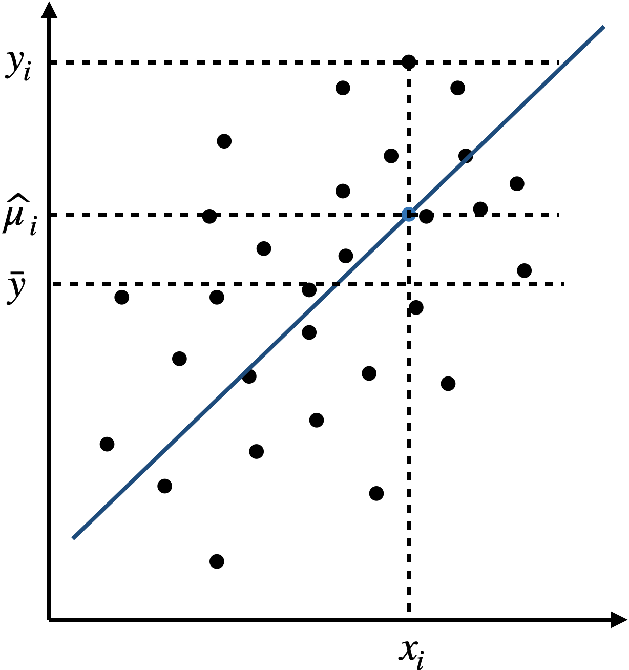
4.4.2.1 ANOVA decomposition for simple linear regression
Figure 4.2 gives an interpretation of the ANOVA decomposition (4.2) in the case of the simple linear regression model (4.4).
4.4.2.2 Connection between \(R^2\) and correlation
There is a connection between \(R^2\) and correlation in simple linear regression.
Proposition 4.3 Let \(\rho_{xy}\) denote the sample correlation between \(x\) and \(y\), and let \(R^2_{xy}\) be the \(R^2\) from the simple linear regression (4.4). Then, we have: \[ R^2 = \rho_{xy}^2. \]
Proof. This fact is a consequence of Proposition 4.2.
4.4.2.3 Regression to the mean
Simple linear regression can be used to study the relationship between the same quantity across time (or generations). For example, let \(x\) and \(y\) be the height of a parent and child. This example motivated Sir Francis Galton to study linear regression in the first place. Alternatively, \(x\) and \(y\) can be a student’s score on a standardized test in two consecutive years, or the number of games won by a given sports team in two consecutive seasons. In this situation, it is reasonable to assume that the sample standard deviations of \(x\) and \(y\) are the same (or to normalize these variables to achieve this). In this case, equations (4.5) and (4.6) simplify to:
\[ \widehat{\beta}_0 = \bar{y} - \rho_{xy} \bar{x} \quad \text{and} \quad \widehat{\beta}_1 = \rho_{xy}. \tag{4.7}\]
It follows that:
\[ |\widehat{\mu}_i - \bar{y}| = |\widehat{\beta}_0 + \widehat{\beta}_1 x_i - \bar{y}| = |\rho_{xy}(x_i - \bar{x})| = |\rho_{xy}| \cdot |x_i - \bar{x}|. \]
Since \(|\rho_{xy}| < 1\) unless \(\boldsymbol{x}\) and \(\boldsymbol{y}\) are perfectly correlated (by the Cauchy-Schwarz inequality), this means that:
\[ |\widehat{\mu}_i - \bar{y}| < |x_i - \bar{x}| \quad \text{for each } i. \tag{4.8}\]
Therefore, we expect \(y_i\) to be closer to its mean than \(x_i\) is to its mean. This phenomenon is called regression to the mean (and is in fact the origin of the term “regression”). Many mistakenly attribute a causal mechanism to this phenomenon, when in reality it is simply a statistical artifact. For example, suppose \(x_i\) is the number of games a sports team won last season and \(y_i\) is the number of games it won this season. It is widely observed that teams with exceptional performance in a given season suffer a “winner’s curse,” performing worse in the next season. The reason for the winner’s curse is simple: teams perform exceptionally well due to a combination of skill and luck. While skill stays roughly constant from year to year, the team which performed exceptionally well in a given season is unlikely to get as lucky as it did the next season.