12  R demo

See also Agresti 3.4.1, 3.4.3, Dunn and Smyth 2.6, 2.14

Let’s put into practice what we’ve learned in this chapter by analyzing data about house prices.

library(tidyverse)
library(GGally)

houses_data <- read_tsv("data/Houses.dat")
houses_data

# A tibble: 100 × 7
    case taxes  beds baths   new price  size
   <dbl> <dbl> <dbl> <dbl> <dbl> <dbl> <dbl>
 1     1  3104     4     2     0  280.  2048
 2     2  1173     2     1     0  146.   912
 3     3  3076     4     2     0  238.  1654
 4     4  1608     3     2     0  200   2068
 5     5  1454     3     3     0  160.  1477
 6     6  2997     3     2     1  500.  3153
 7     7  4054     3     2     0  266.  1355
 8     8  3002     3     2     1  290.  2075
 9     9  6627     5     4     0  587   3990
10    10   320     3     2     0   70   1160
# ℹ 90 more rows

12.1 Exploration

Let’s first do a bit of exploration:

# visualize distribution of housing prices, superimposing the mean
houses_data |>
  ggplot(aes(x = price)) +
  geom_histogram(color = "black", bins = 30) +
  geom_vline(aes(xintercept = mean(price)),
    colour = "red",
    linetype = "dashed"
  )

# compare median and mean price
houses_data |>
  summarise(
    mean_price = mean(price),
    median_price = median(price)
  )

# A tibble: 1 × 2
  mean_price median_price
       <dbl>        <dbl>
1       155.         133.

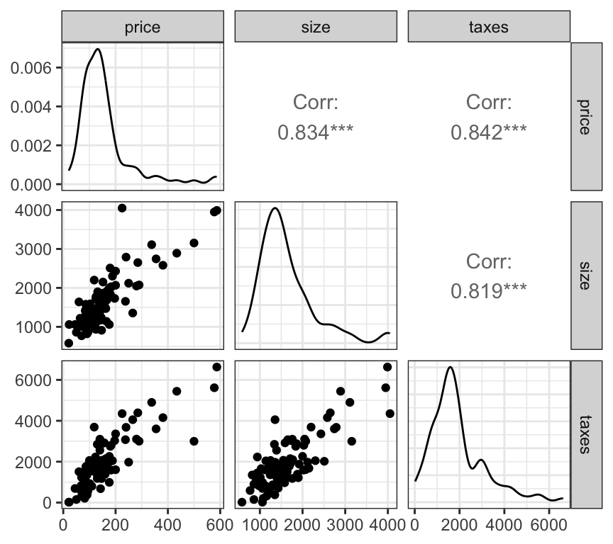
# create a pairs plot of continuous variables
houses_data |>
  select(price, size, taxes) |>
  ggpairs()

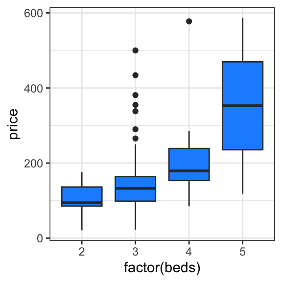
# see how price relates to beds
houses_data |>
  ggplot(aes(x = factor(beds), y = price)) +
  geom_boxplot(fill = "dodgerblue")

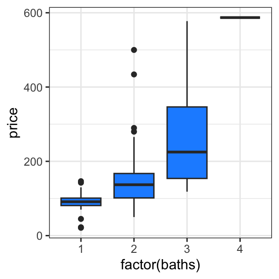
# see how price relates to baths
houses_data |>
  ggplot(aes(x = factor(baths), y = price)) +
  geom_boxplot(fill = "dodgerblue")

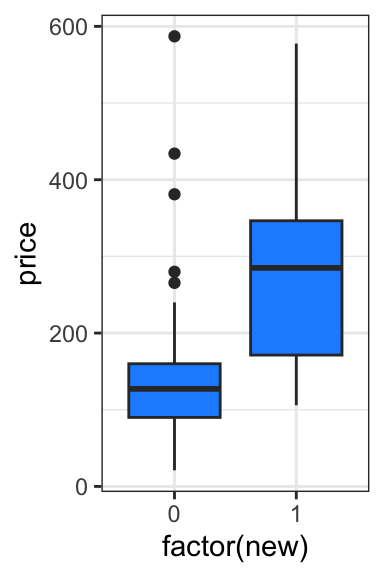
# see how price relates to new
houses_data |>
  ggplot(aes(x = factor(new), y = price)) +
  geom_boxplot(fill = "dodgerblue")

12.2 Hypothesis testing

Let’s run a linear regression and interpret the summary. But first, we must decide whether to model beds/baths as categorical or continuous? We should probably model these as categorical, given the potentially nonlinear trend observed in the box plots.

lm_fit <- lm(price ~ factor(beds) + factor(baths) + new + size,
  data = houses_data
)
summary(lm_fit)

Call:
lm(formula = price ~ factor(beds) + factor(baths) + new + size, 
    data = houses_data)

Residuals:
     Min       1Q   Median       3Q      Max 
-179.306  -32.037   -2.899   19.115  152.718 

Coefficients:
                 Estimate Std. Error t value Pr(>|t|)    
(Intercept)     -19.26307   18.01344  -1.069 0.287730    
factor(beds)3   -16.46430   15.04669  -1.094 0.276749    
factor(beds)4   -12.48561   21.12357  -0.591 0.555936    
factor(beds)5  -101.14581   55.83607  -1.811 0.073366 .  
factor(baths)2    2.39872   15.44014   0.155 0.876885    
factor(baths)3   -0.70410   26.45512  -0.027 0.978825    
factor(baths)4  273.20079   83.65764   3.266 0.001540 ** 
new              66.94940   18.50445   3.618 0.000487 ***
size              0.10882    0.01234   8.822 7.46e-14 ***
---
Signif. codes:  0 '***' 0.001 '**' 0.01 '*' 0.05 '.' 0.1 ' ' 1

Residual standard error: 51.17 on 91 degrees of freedom
Multiple R-squared:  0.7653,    Adjusted R-squared:  0.7446 
F-statistic: 37.08 on 8 and 91 DF,  p-value: < 2.2e-16

We can read off the test statistics and \(p\)-values for each variable from the regression summary, as well as for the \(F\)-test against the constant model from the bottom of the summary.

Let’s use an \(F\)-test to assess whether the categorical baths variable is important.

lm_fit_partial <- lm(price ~ factor(beds) + new + size,
  data = houses_data
)
anova(lm_fit_partial, lm_fit)

Analysis of Variance Table

Model 1: price ~ factor(beds) + new + size
Model 2: price ~ factor(beds) + factor(baths) + new + size
  Res.Df    RSS Df Sum of Sq      F   Pr(>F)   
1     94 273722                                
2     91 238289  3     35433 4.5104 0.005374 **
---
Signif. codes:  0 '***' 0.001 '**' 0.01 '*' 0.05 '.' 0.1 ' ' 1

What if we had not coded baths as a factor?

lm_fit_not_factor <- lm(price ~ factor(beds) + baths + new + size,
  data = houses_data
)
anova(lm_fit_partial, lm_fit_not_factor)

Analysis of Variance Table

Model 1: price ~ factor(beds) + new + size
Model 2: price ~ factor(beds) + baths + new + size
  Res.Df    RSS Df Sum of Sq      F Pr(>F)
1     94 273722                           
2     93 273628  1     94.33 0.0321 0.8583

If we want to test for the equality of means across groups of a categorical predictor, without adjusting for other variables, we can use the ANOVA \(F\)-test. There are several equivalent ways of doing so:

# just use the summary function
lm_fit_baths <- lm(price ~ factor(baths), data = houses_data)
summary(lm_fit_baths)

Call:
lm(formula = price ~ factor(baths), data = houses_data)

Residuals:
    Min      1Q  Median      3Q     Max 
-146.44  -45.88   -7.89   22.22  352.01 

Coefficients:
               Estimate Std. Error t value Pr(>|t|)    
(Intercept)       90.21      19.51   4.624 1.17e-05 ***
factor(baths)2    57.68      21.72   2.656  0.00927 ** 
factor(baths)3   174.52      31.13   5.607 1.97e-07 ***
factor(baths)4   496.79      82.77   6.002 3.45e-08 ***
---
Signif. codes:  0 '***' 0.001 '**' 0.01 '*' 0.05 '.' 0.1 ' ' 1

Residual standard error: 80.44 on 96 degrees of freedom
Multiple R-squared:  0.3881,    Adjusted R-squared:  0.369 
F-statistic:  20.3 on 3 and 96 DF,  p-value: 2.865e-10

# use the anova function as before
lm_fit_const <- lm(price ~ 1, data = houses_data)
anova(lm_fit_const, lm_fit_baths)

Analysis of Variance Table

Model 1: price ~ 1
Model 2: price ~ factor(baths)
  Res.Df     RSS Df Sum of Sq      F    Pr(>F)    
1     99 1015150                                  
2     96  621130  3    394020 20.299 2.865e-10 ***
---
Signif. codes:  0 '***' 0.001 '**' 0.01 '*' 0.05 '.' 0.1 ' ' 1

# use the aov function
aov_fit <- aov(price ~ factor(baths), data = houses_data)
summary(aov_fit)

              Df Sum Sq Mean Sq F value   Pr(>F)    
factor(baths)  3 394020  131340    20.3 2.86e-10 ***
Residuals     96 621130    6470                     
---
Signif. codes:  0 '***' 0.001 '**' 0.01 '*' 0.05 '.' 0.1 ' ' 1

We can also use an \(F\)-test to test for the presence of an interaction with a multi-class categorical predictor.

lm_fit_interaction <- lm(price ~ size * factor(beds), data = houses_data)
summary(lm_fit_interaction)

Call:
lm(formula = price ~ size * factor(beds), data = houses_data)

Residuals:
     Min       1Q   Median       3Q      Max 
-232.643  -25.938   -0.942   19.172  155.517 

Coefficients:
                     Estimate Std. Error t value Pr(>|t|)    
(Intercept)          50.12619   48.22282   1.039 0.301310    
size                  0.05037    0.04210   1.197 0.234565    
factor(beds)3      -103.85734   52.20373  -1.989 0.049620 *  
factor(beds)4      -143.90213   67.31359  -2.138 0.035185 *  
factor(beds)5      -507.88205  144.10191  -3.524 0.000663 ***
size:factor(beds)3    0.07589    0.04368   1.738 0.085633 .  
size:factor(beds)4    0.09234    0.04704   1.963 0.052638 .  
size:factor(beds)5    0.21147    0.05957   3.550 0.000609 ***
---
Signif. codes:  0 '***' 0.001 '**' 0.01 '*' 0.05 '.' 0.1 ' ' 1

Residual standard error: 53.35 on 92 degrees of freedom
Multiple R-squared:  0.7421,    Adjusted R-squared:  0.7225 
F-statistic: 37.81 on 7 and 92 DF,  p-value: < 2.2e-16

lm_fit_size <- lm(price ~ size + factor(beds), data = houses_data)
anova(lm_fit_size, lm_fit_interaction)

Analysis of Variance Table

Model 1: price ~ size + factor(beds)
Model 2: price ~ size * factor(beds)
  Res.Df    RSS Df Sum of Sq      F   Pr(>F)   
1     95 300953                                
2     92 261832  3     39121 4.5819 0.004905 **
---
Signif. codes:  0 '***' 0.001 '**' 0.01 '*' 0.05 '.' 0.1 ' ' 1

Contrasts of regression coefficients can be tested using the glht() function from the multcomp package.

12.3 Confidence intervals

We can construct pointwise confidence intervals for each coefficient using confint():

confint(lm_fit)

                       2.5 %      97.5 %
(Intercept)     -55.04455734  16.5184161
factor(beds)3   -46.35270691  13.4241025
factor(beds)4   -54.44498235  29.4737689
factor(beds)5  -212.05730801   9.7656895
factor(baths)2  -28.27123130  33.0686620
factor(baths)3  -53.25394742  51.8457394
factor(baths)4  107.02516067 439.3764122
new              30.19258305 103.7062177
size              0.08431972   0.1333284

To create simultaneous confidence intervals, we need a somewhat more manual approach. We start with the coefficients and standard errors:

coef(summary(lm_fit))

                   Estimate  Std. Error     t value     Pr(>|t|)
(Intercept)     -19.2630706 18.01344052 -1.06937209 2.877304e-01
factor(beds)3   -16.4643022 15.04669172 -1.09421410 2.767490e-01
factor(beds)4   -12.4856067 21.12356937 -0.59107467 5.559357e-01
factor(beds)5  -101.1458092 55.83607248 -1.81147786 7.336590e-02
factor(baths)2    2.3987153 15.44014266  0.15535578 8.768849e-01
factor(baths)3   -0.7041040 26.45511871 -0.02661504 9.788251e-01
factor(baths)4  273.2007864 83.65764044  3.26570036 1.540093e-03
new              66.9494004 18.50445029  3.61801617 4.872475e-04
size              0.1088241  0.01233621  8.82151661 7.460814e-14

Then we add lower and upper confidence interval endpoints based on the formula (10.9):

alpha <- 0.05
n <- nrow(houses_data)
p <- length(coef(lm_fit))
f_quantile <- qf(1 - alpha, df1 = p, df2 = n - p)
coef(summary(lm_fit)) |>
  as.data.frame() |>
  rownames_to_column(var = "Variable") |>
  select(Variable, Estimate, `Std. Error`) |>
  mutate(
    CI_lower = Estimate - `Std. Error` * sqrt(p * f_quantile),
    CI_upper = Estimate + `Std. Error` * sqrt(p * f_quantile)
  )

        Variable     Estimate  Std. Error      CI_lower    CI_upper
1    (Intercept)  -19.2630706 18.01344052  -95.38917389  56.8630327
2  factor(beds)3  -16.4643022 15.04669172  -80.05271036  47.1241059
3  factor(beds)4  -12.4856067 21.12356937 -101.75533960  76.7841262
4  factor(beds)5 -101.1458092 55.83607248 -337.11309238 134.8214739
5 factor(baths)2    2.3987153 15.44014266  -62.85244495  67.6498756
6 factor(baths)3   -0.7041040 26.45511871 -112.50535022 111.0971422
7 factor(baths)4  273.2007864 83.65764044  -80.34245635 626.7440292
8            new   66.9494004 18.50445029  -11.25174573 145.1505465
9           size    0.1088241  0.01233621    0.05669037   0.1609578

Note that the simultaneous intervals are substantially larger.

To construct pointwise confidence intervals for the fit, we can use the predict() function:

predict(lm_fit, newdata = houses_data, interval = "confidence") |> head()

        fit       lwr      upr
1 193.52176 165.22213 221.8214
2  79.98449  51.91430 108.0547
3 150.64507 122.28397 179.0062
4 191.71955 172.27396 211.1651
5 124.30169  81.34488 167.2585
6 376.74308 333.44559 420.0406

To get pointwise prediction intervals, we switch "confidence" to "prediction":

predict(lm_fit, newdata = houses_data, interval = "prediction") |> head()

        fit       lwr      upr
1 193.52176  88.00908 299.0344
2  79.98449 -25.46688 185.4359
3 150.64507  45.11589 256.1743
4 191.71955  88.22951 295.2096
5 124.30169  13.95069 234.6527
6 376.74308 266.25901 487.2271

To construct simultaneous confidence intervals for the fit or predictions, we again need a slightly more manual approach. We call predict() again, but this time asking it for the standard errors rather than the confidence intervals:

predictions <- predict(lm_fit, newdata = houses_data, se.fit = TRUE)
head(predictions$fit)

        1         2         3         4         5         6 
193.52176  79.98449 150.64507 191.71955 124.30169 376.74308 

head(predictions$se.fit)

        1         2         3         4         5         6 
14.246855 14.131352 14.277804  9.789472 21.625709 21.797212 

Now we can construct the simultaneous confidence intervals via the formula (10.8):

f_quantile <- qf(1 - alpha, df1 = p, df2 = n - p)
tibble(
  lower = predictions$fit - predictions$se.fit * sqrt(p * f_quantile),
  upper = predictions$fit + predictions$se.fit * sqrt(p * f_quantile)
)

# A tibble: 100 × 2
   lower upper
   <dbl> <dbl>
 1 133.   254.
 2  20.3  140.
 3  90.3  211.
 4 150.   233.
 5  32.9  216.
 6 285.   469.
 7  82.8  145.
 8 188.   331.
 9 371.   803.
10  57.3  128.
# ℹ 90 more rows

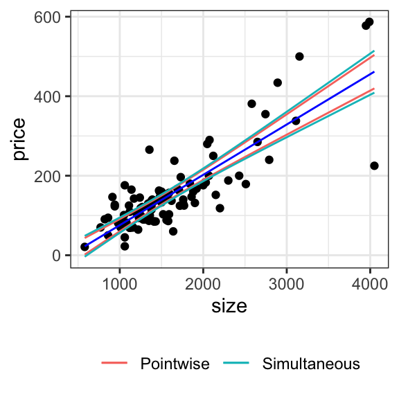
In the case of simple linear regression, we can plot these pointwise and simultaneous confidence intervals as bands:

# to produce confidence intervals for fits in general, use the predict() function
n <- nrow(houses_data)
p <- 2
alpha <- 0.05
lm_fit <- lm(price ~ size, data = houses_data)
predictions <- predict(lm_fit, se.fit = TRUE)
t_quantile <- qt(1 - alpha / 2, df = n - p)
f_quantile <- qf(1 - alpha, df1 = p, df2 = n - p)
houses_data |>
  mutate(
    fit = predictions$fit,
    se = predictions$se.fit,
    ptwise_width = t_quantile * se,
    simultaneous_width = sqrt(p * f_quantile) * se
  ) |>
  ggplot(aes(x = size)) +
  geom_point(aes(y = price)) +
  geom_line(aes(y = fit), color = "blue") +
  geom_line(aes(y = fit + ptwise_width, color = "Pointwise")) +
  geom_line(aes(y = fit - ptwise_width, color = "Pointwise")) +
  geom_line(aes(y = fit + simultaneous_width, color = "Simultaneous")) +
  geom_line(aes(y = fit - simultaneous_width, color = "Simultaneous")) +
  theme(legend.title = element_blank(), legend.position = "bottom")

12.4 Predictor competition and collaboration

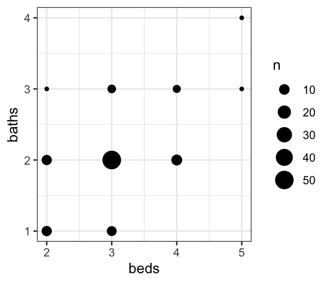
Let’s look at the power of detecting the association between price and beds. We can imagine that beds and baths are correlated:

houses_data |>
  ggplot(aes(x = beds, y = baths)) +
  geom_count()

So let’s see how significant beds is, with and without baths in the model:

lm_fit_only_beds <- lm(price ~ factor(beds), data = houses_data)
summary(lm_fit_only_beds)

Call:
lm(formula = price ~ factor(beds), data = houses_data)

Residuals:
    Min      1Q  Median      3Q     Max 
-234.35  -50.63  -15.69   24.56  365.86 

Coefficients:
              Estimate Std. Error t value Pr(>|t|)    
(Intercept)     105.94      21.48   4.931 3.43e-06 ***
factor(beds)3    44.69      24.47   1.827 0.070849 .  
factor(beds)4   105.70      32.35   3.268 0.001504 ** 
factor(beds)5   246.71      69.62   3.544 0.000611 ***
---
Signif. codes:  0 '***' 0.001 '**' 0.01 '*' 0.05 '.' 0.1 ' ' 1

Residual standard error: 93.65 on 96 degrees of freedom
Multiple R-squared:  0.1706,    Adjusted R-squared:  0.1447 
F-statistic: 6.583 on 3 and 96 DF,  p-value: 0.0004294

lm_fit_only_baths <- lm(price ~ factor(baths), data = houses_data)
lm_fit_beds_baths <- lm(price ~ factor(beds) + factor(baths), data = houses_data)
anova(lm_fit_only_baths, lm_fit_beds_baths)

Analysis of Variance Table

Model 1: price ~ factor(baths)
Model 2: price ~ factor(beds) + factor(baths)
  Res.Df    RSS Df Sum of Sq     F  Pr(>F)  
1     96 621130                             
2     93 572436  3     48693 2.637 0.05424 .
---
Signif. codes:  0 '***' 0.001 '**' 0.01 '*' 0.05 '.' 0.1 ' ' 1

We see that the significance of beds dropped by two orders of magnitude. This is an example of predictor competition.

On the other hand, note that the variable new is not very correlated with beds:

lm_fit <- lm(new ~ beds, data = houses_data)
summary(lm_fit)

Call:
lm(formula = new ~ beds, data = houses_data)

Residuals:
     Min       1Q   Median       3Q      Max 
-0.15762 -0.11000 -0.11000 -0.08619  0.91381 

Coefficients:
            Estimate Std. Error t value Pr(>|t|)
(Intercept)  0.03857    0.14950   0.258    0.797
beds         0.02381    0.04871   0.489    0.626

Residual standard error: 0.3157 on 98 degrees of freedom
Multiple R-squared:  0.002432,  Adjusted R-squared:  -0.007747 
F-statistic: 0.2389 on 1 and 98 DF,  p-value: 0.6261

but we know it has a substantial impact on price. Let’s look at the significance of the test that beds is not important when we add new to the model.

lm_fit_only_new <- lm(price ~ new, data = houses_data)
lm_fit_beds_new <- lm(price ~ new + factor(beds), data = houses_data)
anova(lm_fit_only_new, lm_fit_beds_new)

Analysis of Variance Table

Model 1: price ~ new
Model 2: price ~ new + factor(beds)
  Res.Df    RSS Df Sum of Sq      F    Pr(>F)    
1     98 787781                                  
2     95 619845  3    167936 8.5795 4.251e-05 ***
---
Signif. codes:  0 '***' 0.001 '**' 0.01 '*' 0.05 '.' 0.1 ' ' 1

Adding new to the model made the \(p\)-value more significant by a factor of 10. This is an example of predictor collaboration.